


Week 04 · Complete notes
Monopolistic markets
How should a firm act when it can control the price?
This print edition combines all five readings. Interactive definitions become ordinary text when printed.
01
Market power
What does it take for a firm to set its own price?
In competitive markets, no firm chose its price. Each Auto Eco firm took the market price as given and decided only how much to produce. Even Portakal's island farms, which kept earning a profit, couldn't charge a cent above the market price. If one of them had tried, buyers would have bought from the other forty-nine.
This week we study a firm that serves the whole market, so the market's demand curve is its own demand curve. That single change has a large consequence. If the firm wants to sell more, it has to charge less, and if it wants to charge more, it has to sell less.
This first reading sets up the model. We ask what gives a firm this kind of power, how durable the power is, and how the firm chooses its price and quantity. We also meet Ride On, the example we'll follow through the whole week.
1.1
What makes a monopoly
A is a market served by a single seller of a good with no close substitutes, protected by an entry barrier that keeps other firms out. Each of the three assumptions is crucial, and it helps to see what goes wrong when one of them is missing.
Suppose there's only one seller, but buyers have a close substitute. Say the only bakery in a small town is the only place to buy bread. But the supermarket down the road sells tortillas, and many customers see tortillas as a substitute for bread. Then the bakery can't raise its bread price much before customers switch. Being the only seller of a good isn't enough. The firm needs to be the only seller of something buyers can't easily replace.
Now suppose there's one seller and no close substitute, but nothing stops others from entering. Then the situation is temporary. In Week 3, Auto Eco's profit of $24 million a month attracted new firms, and they kept coming until the profit was gone. A monopolist earning a profit faces the same pressure. It stays a monopolist only as long as something stops that entry from happening. We called this an entry barrier in Week 3.
So a monopoly needs all three assumptions at once.
1.2
Where barriers come from
Barriers come in three broad kinds. Naming the kind tells you how long the position is likely to last, and that's usually the first thing a manager or an investor wants to know.
Legal barriers. Patents, copyright, licenses and exclusive contracts all give one firm the legal right to sell and forbid others. A drug company with a patent on a new medicine is the standard example. The state creates these barriers and the state can remove them. A patent expires after a fixed term, and a license can be withdrawn or issued to a rival. So legal barriers can be very strong, but they last only as long as the law protects them.
Structural barriers. Sometimes the barrier comes from the economics of the industry itself. One firm may control a scarce input, such as the only quarry with a particular stone. Or the cost structure may make one firm cheaper than two. A water network, an electricity grid or a railway costs a great deal to build once and very little to run for one more customer. Building a second network beside the first would double the large cost and split the same customers. When one firm has an overwhelming cost advantage over competitors, we call it a . Structural barriers last as long as the cost advantage lasts.
Strategic barriers. An incumbent can also behave in ways that make entry unattractive, for example by building more capacity than it needs so that an entrant expects a price war. Whether a threat like that works depends on whether the entrant believes it. That's a question about strategy, and it needs the game theory of Weeks 6 to 8. We come back to it in Week 8.
The table at the end of Week 3 asked where persistent profit comes from. Every row of that table, from scarce land to patents, is also a source of market power. The difference this week is that the barrier protects a single firm rather than a group of price-taking firms.
1.3
Market power is a matter of degree
Very few firms are literal monopolies. Many more have some : they can raise their price and lose some customers rather than all of them. That's all this week's model needs.
Apple is a useful example. It isn't the only maker of phones, and Samsung, Google and others sell close alternatives. Yet when Apple raises the price of an iPhone a little, demand doesn't collapse. Many customers have bought apps, stored years of photos and messages, and learned how the system works. Switching to another phone would cost them time and money, and some of what they've built up would be lost. Those switching costs, together with the features that set the iPhone apart from other phones, give Apple a downward-sloping demand curve of its own, even in a market with strong rivals.
So the monopoly model applies to any firm whose own demand slopes down. What matters is not the firm's share of some broadly defined market. What matters is how easily its customers can find a substitute when its price rises.
1.4
Price and quantity become one decision
Recall how Week 2 described a price-taker. Auto Eco could sell as many vehicles as it wanted at the market price, and none at all above it. Its demand curve, the demand for its own output, was a horizontal line at the market price. So its only decision was how much to produce.
A monopolist faces the whole market demand curve instead. It chooses a point on that curve, a pair of price and quantity, to maximize its profit. Choosing a price and choosing a quantity are the same thing. If the monopolist sets the price, the demand curve tells it how many units it sells. If it sets the quantity, the demand curve tells it the price at which those units sell. So for a monopolist, price and quantity are one decision.
Our main example this week is Ride On. Ride On operates the coin-operated children's rides in a shopping mall. Inside the mall it has no competitor. Its daily demand is
where \(Q\) is the number of rides per day and \(p\) is the price of a ride in dollars. At a price of $3, children take \(140-120=20\) rides a day. At $2, they take 60. At $1, they take 100. Ride On can choose any of these combinations. What it can't do is sell 60 rides at $3, because at $3 only 20 children want a ride.
Since the monopolist's output is the whole market's output, we write it with a capital \(Q\), as we did for market quantities in Weeks 2 and 3. We'll describe Ride On's choice in terms of quantity: how many rides to sell. That makes the comparison with Auto Eco easy, because Auto Eco also chose a quantity. Nothing depends on this choice. Choosing 60 rides and choosing a price of $2 are the same decision.
1.5
Ride On's cost and inverse demand
Ride On's daily economic cost is
The 40 is the daily rental Ride On pays the mall for its space. The 0.5 is the cost of one more ride: electricity and the wear on the machines. Ride On can end the rental if it closes the rides, so the whole of \(C(Q)\) is avoidable, as in our cost functions from Week 1. Marginal cost is constant at 50 cents a ride.
The demand function answers the question: at this price, how many rides do children want? A monopolist choosing a quantity needs the reverse. If I want to sell this many rides, what's the highest price I can charge? Writing price in terms of quantity demanded answers this question. It's called the function, \(p(Q)\). For Ride On, solve the demand equation for \(p\):
You can read it as a price list. To sell 60 rides a day, Ride On can charge \(p(60)=3.5-60/40=2\) dollars. To sell 100, it has to drop to \(p(100)=1\) dollar. At $3.50 no child rides at all.
There's a second way to read the same function, and it connects back to Week 1. Market demand adds up individual buyers, as we saw in Week 2. Assume each child takes at most one ride. Line the children up from the highest willingness to pay to the lowest. Then \(p(Q)\) is the WTP of the \(Q\)th child in line. The 60th child values a ride at exactly $2. Every child ahead of them values it at more, and every child behind them at less. That's why the price must fall to sell more: the next customer always values a ride a little less than the last one.
For any linear demand \(Q^d(p)=a-bp\) with \(a,b>0\), the same steps give
The intercept \(a/b\) is the price at which demand falls to zero. The slope \(-1/b\) is how much the price must fall to sell one more unit.
1.6
What the monopoly model does and doesn't claim
The model says that a firm with market power chooses a point on its demand curve to maximize its profit. It can set any price it likes, but then demand decides how many units it sells. It doesn't claim that a monopolist can charge whatever it likes. Ride On could post a price of $10 tomorrow, but no child would ride.
It also doesn't claim that monopolists are large, or that they behave badly. A single ride operator in one mall and a pharmaceutical company with a blockbuster patent face the same pricing problem with very different market conditions.
The model does make two assumptions that we'll keep this week and relax later. First, the firm charges one market price. Ride On charges one price per ride, whoever is riding. In Week 5 we ask what a firm can do when it can charge different buyers different prices. Second, the firm knows its demand curve. In practice firms estimate demand from market data. Throughout the course, when a problem gives you a demand function, you can take it as the result of that kind of careful estimation.
Summary. A monopoly needs one seller, no close substitutes and a barrier to entry, which can be legal, structural or strategic. Market power is a matter of degree: any firm with a demand for its product can adjust its price without losing every customer. Such a firm chooses a point on its demand curve, a pair of price and quantity, so price and quantity are a single decision. Inverse demand \(p(Q)\) gives the price at which \(Q\) units sell, which is also the WTP of the \(Q\)th buyer.
02
Marginal revenue
What does one more sale really add to revenue?
In Week 2, every vehicle Auto Eco sold brought in the market price. So one more vehicle added exactly the same price to revenue, and Auto Eco expanded until marginal cost reached the price.
Ride On can't sell one more ride at the current price. To sell it, Ride On must lower the price, and because every child pays the same price, it lowers the price on every ride. So one more ride adds its price to revenue, but it also takes something away: the discount on all the rides that would have sold anyway.
This reading measures that discount. The measure is called marginal revenue, and it does for the revenue side what marginal cost does for the cost side.
2.1
Total and average revenue
is the price times the quantity sold. For a firm with market power, the price depends on the quantity, so
For Ride On,
Revenue is quadratic in \(Q\), just like the quadratic cost functions in Week 1. Move the point along demand in the top panel and watch revenue change in the bottom panel.
Revenue rises at first, peaks at 70 rides and then falls. Selling more rides isn't always good for revenue, because selling more means charging less. Past 70 rides, the lower price costs more than the extra rides bring in.
is revenue per unit, \(R(Q)/Q\). Every ride sells at the same price, so average revenue is simply the price, \(p(Q)\). In other words, the demand curve is the average-revenue curve.
2.2
Selling more means a discount on every unit
Suppose Ride On sells 40 rides a day at $2.50 and considers selling 50 instead. To sell 50 rides, the price must fall to \(p(50)=2.25\). Revenue changes for two reasons.
New revenue. The ten extra rides each sell for $2.25. That adds \(10\times2.25=22.50\) dollars.
Lost revenue. The 40 children who were already riding at $2.50 now pay $2.25 too. Each pays 25 cents less, so Ride On loses \(40\times0.25=10\) dollars on rides it would have sold anyway.
So revenue rises by \(22.50-10=12.50\), from $100 to $112.50. The ten extra rides bring in $22.50, but the net gain is only $12.50. The difference is the discount Ride On has to give its existing customers.
is the change in total revenue from selling one more unit. Over this step, revenue rises by $12.50 for ten extra rides, or about $1.25 per extra ride. Each extra ride sells for $2.25, but adds only about $1.25 to revenue. The gap between the price and marginal revenue is the cost of the discount.
The same logic works for any change in quantity. Start from a price and quantity pair \((p,Q)\) on the demand curve. Suppose the firm sells \(\Delta Q\) more units. To sell them, the price has to change by \(\Delta p\), so it goes from \(p\) to \(p+\Delta p\). Demand slopes down, so \(\Delta p\) is negative. Quantity goes from \(Q\) to \(Q+\Delta Q\).
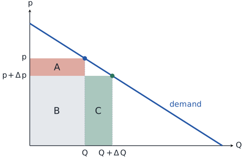
Before the change, revenue is \(p\times Q\), the area \(A+B\). After the change, revenue is \((p+\Delta p)\times(Q+\Delta Q)\), the area \(B+C\). Area \(B\) is in both, so the change in revenue is
Area \(C\) is the new revenue: \(\Delta Q\) extra units, each sold at the new price \(p+\Delta p\). Area \(A\) is the lost revenue: the \(Q\) units that would have sold anyway now sell for \(-\Delta p\) less each. We write \(-\Delta p\) because \(\Delta p\) is negative and an area has to be positive.
Marginal revenue is the change in revenue for each extra unit, so we divide the change in revenue by \(\Delta Q\):
If revenue is continuous in \(Q\), we can make the change in \(Q\) infinitesimally small. As \(\Delta Q\) tends to zero, \(\Delta p\) also tends to zero, and the formula becomes
The first part, \(p+\Delta p\), is the price at which the extra units sell. The second part, \(Q\times\Delta p/\Delta Q\), is the discount on the units that would have sold anyway, for each extra unit. It's negative, because \(\Delta p/\Delta Q\) is negative.
Check it with Ride On's step from 40 to 50 rides. Here \(p+\Delta p=2.25\), \(Q=40\) and \(\Delta p/\Delta Q=-0.25/10=-0.025\), so
which is the $1.25 per extra ride we found above. In the graph below, \(A\) is the red strip, \(B\) is the gray area and \(C\) is the green strip.
As you move right, the red strip gets longer. The price cut needed to sell ten more rides is always 25 cents, but it applies to more and more existing rides. At the same time the green strip gets shorter, because the extra rides sell at a lower and lower price. Eventually the lost revenue catches up with the new revenue, and after that it's larger.
Predict before you move the graph
Ride On currently sells 80 rides a day. It considers lowering the price to sell 90. What happens to revenue?
Revenue falls by $7.50. The price drops from $1.50 to $1.25. The ten extra rides add \(10\times1.25=12.50\), but the 80 existing rides each lose 25 cents, which costs \(80\times0.25=20\). Past 70 rides, the discount on existing sales outweighs the new sales.
2.3
Marginal revenue
The ten-ride step gives an approximation. To find marginal revenue exactly, we apply the same method to revenue that we applied to cost in Week 1. Ride On's revenue, \(R(Q)=3.5Q-Q^2/40\), has the same form as the quadratic cost function \(C(q)=a+bq+cq^2\), with \(a=0\), \(b=3.5\) and \(c=-1/40\). In Week 1, marginal cost was \(b+2cq\). So for Ride On,
Check it against the ten-ride step. The step from 40 to 50 rides averaged $1.25 per ride. Marginal revenue at the middle of that step, 45 rides, is \(MR(45)=3.5-45/20=1.25\). The two methods agree exactly here because revenue is quadratic, so its slope changes at a constant rate.
The general version shows where the gap between price and marginal revenue comes from. For any demand curve, marginal revenue is
Each term matches one of the strips. The first term, \(p(Q)\), is the new revenue: the price the extra unit sells for. The second term is the lost revenue. Here \(dp/dQ\) is how much the price must change to sell one more unit, and it applies to all \(Q\) units already being sold. Demand slopes down, so \(dp/dQ\) is negative, the second term is negative, and marginal revenue is below the price at every positive output.
Demand for the firm's output is flat at the market price, so \(dp/dQ=0\) and \(MR(Q)=p\).
Demand slopes down, so \(dp/dQ\lt 0\) and \(MR(Q)\lt p\).
So Week 2's rule, expand until price equals marginal cost, was really "expand until marginal revenue equals marginal cost" for a firm whose marginal revenue happens to equal the price.
2.4
The linear rule
Most problems in this course use linear demand, so one shortcut is worth remembering. If inverse demand is \(p(Q)=a-bQ\), then
Marginal revenue has the same intercept as inverse demand and twice the slope. So the marginal-revenue line starts at the same point on the price axis and falls twice as fast. It reaches zero halfway to the quantity at which demand reaches zero.
For Ride On, \(a=3.5\) and \(b=1/40\), so \(MR(Q)=3.5-Q/20\), which matches what we found above. Demand reaches zero at 140 rides and marginal revenue reaches zero at 70.
That point at 70 rides matters. Below 70, marginal revenue is positive and selling one more ride raises revenue. Above 70, marginal revenue is negative and selling one more ride lowers revenue. At exactly 70, revenue is at its peak of $122.50, which is what the graph showed.
2.5
Marginal revenue isn't the price of the last unit
The most common error with marginal revenue is to treat it as the price at which the last unit sells. At 40 rides, the 40th ride sells for $2.50. But marginal revenue at 40 rides is \(MR(40)=3.5-40/20=1.50\), a dollar less. The extra ride brings in $2.50 from the child who takes it, and costs Ride On a small discount on the 39 rides it was already selling.
So it helps to keep the two curves apart. The demand curve tells you what the next buyer pays. The marginal-revenue curve tells you what the next sale adds to the firm's revenue. For a price-taker the two are the same. For a firm with market power they aren't, and the gap grows as output grows, because the discount applies to more and more units.
There's a managerial version of the same point. A sales team that counts the revenue from each new customer at the price that customer pays will overstate what the extra sales are worth whenever winning those customers requires a lower price for everyone.
Summary. Total revenue is \(R(Q)=p(Q)\times Q\), and the demand curve is the average-revenue curve. Selling one more unit brings in its price but lowers the price on every unit that would have sold anyway, so marginal revenue lies below price. With linear inverse demand \(p(Q)=a-bQ\), \(MR=a-2bQ\): same intercept, twice the slope. Revenue peaks where marginal revenue is zero, at 70 rides for Ride On.
03
Choosing price and output
How does a firm with market power choose its price?
We now have both halves of the comparison. Marginal cost, from Week 1, tells Ride On what one more ride adds to cost. Marginal revenue, from the last reading, tells it what one more ride adds to revenue.
The monopolist's question is the same one Auto Eco asked in Week 2: should I sell one more unit? The logic doesn't change. Only the revenue side does, because Ride On's revenue from one more ride is marginal revenue rather than the price.
We'll find Ride On's best output and price, and then look at what the answer says about price and cost, the most common errors, what happens when costs change, and what happens when the firm can't produce as much as it wants.
3.1
Expand while marginal revenue exceeds marginal cost
Profit is revenue minus economic cost, \(\pi(Q)=R(Q)-C(Q)\). Rather than search every output, pick one and ask whether Ride On could do better by moving.
Start at 40 rides. Marginal revenue is \(MR(40)=3.5-2=1.50\), and marginal cost is 0.50. One more ride adds about $1.50 to revenue and 50 cents to cost, so it adds about $1 to profit. Ride On is leaving money on the table, and it should expand.
Start at 80 rides. Marginal revenue is \(MR(80)=3.5-4=-0.50\). One more ride now lowers revenue by about 50 cents and still costs 50 cents to run. Going the other way, one ride fewer raises revenue by about 50 cents and saves 50 cents of cost, so profit rises by about $1. Ride On should contract.
The same comparison works at any output.
- If \(MR(Q)>MC(Q)\), the next unit adds more to revenue than to cost. Expanding raises profit.
- If \(MR(Q)\lt MC(Q)\), the last unit added more to cost than to revenue. Contracting raises profit.
- If \(MR(Q)=MC(Q)\), neither change helps. Profit is at its peak.
Put differently, the change in profit from one more unit is \(MR(Q)-MC(Q)\), and profit peaks where that change is zero. This gives the :
Choose the output \(Q^m\) at which marginal revenue equals marginal cost. Then charge the price \(p^m\) that demand allows for that output. The superscript \(m\) marks the monopoly choice.
For a price-taker, marginal revenue is the price, so the same rule becomes \(p=MC\), the condition we used for Auto Eco in Week 2. It's one rule, applied to two different revenue curves.
3.2
Ride On, worked through
Ride On's marginal revenue is \(MR(Q)=3.5-Q/20\), and its marginal cost from \(C(Q)=40+0.5Q\) is 0.5 at every output.
Step 1. Set marginal revenue equal to marginal cost.
Step 2. Read the price off demand. Go up from 60 rides to the demand curve, not to the marginal-revenue curve:
Step 3. Calculate profit.
Step 4. Check that the firm should operate at all. As in Week 2, the marginal rule finds the best output if the firm operates. It doesn't say whether operating is better than shutting down. If Ride On shuts down, it saves its whole cost, including the rental, and earns nothing, so its profit is zero. Operating earns $50 a day, so Ride On should operate.
So Ride On sells 60 rides a day at $2 each and earns a daily economic profit of $50.
3.3
Two things the answer says
Price is above marginal cost. At 60 rides, marginal cost is 50 cents, but the price is $2. This isn't a quirk of Ride On's numbers. At the optimum, marginal revenue equals marginal cost. Marginal revenue is below the price, as we saw in the last reading. So the price must be above marginal cost. A monopolist keeps a margin over marginal cost that no price-taker can. Reading 5 shows what determines how large that margin is.
Price is not as high as possible. It's tempting to think a monopolist charges whatever it can get away with. At $3 a ride, Ride On would sell only 20 rides and earn \(3\times20-(40+0.5\times20)=10\) dollars a day. A higher price means a larger margin on each ride but fewer rides. Ride On has to balance the margin on each ride against the number of rides, and the demand curve tells it how many rides it loses when it raises the price.
3.4
The most common errors
The first error is to use the competitive rule. Setting \(p=MC=0.5\) gives \(Q=140-40\times0.5=120\) rides. Revenue is \(0.5\times120=60\) and cost is \(40+0.5\times120=100\), so Ride On would lose $40 a day, exactly its rental. The competitive rule fails here because Ride On isn't a price-taker. It can sell 120 rides only by charging every child 50 cents.
The second error is to read the price off the wrong curve. At \(Q^m=60\), marginal revenue equals 0.5. That's the value of marginal cost, not the price. The price comes from the demand curve. On the graph, go up from 60 rides past the point where \(MR\) meets \(MC\), all the way to demand.
The third error is to think that a fixed cost, such as the rental, should change the price. A fixed cost is the same at every output, so it doesn't change marginal cost. It changes profit, but not the output where \(MR=MC\). Try it with a question.
Check the logic
The mall raises Ride On's daily rental from $40 to $60. Electricity, maintenance and demand don't change. What should Ride On do?
The rental doesn't change marginal revenue or marginal cost, so \(MR=MC\) still holds at 60 rides and \(p=2\). Any other price would lower profit, with or without the higher rent. Profit falls from $50 to $30. It's still positive, so Ride On keeps operating. A cost that doesn't vary with output can change whether a firm operates, but not how much it sells when it does.
3.5
When marginal cost changes
A change in marginal cost is different. Suppose the electricity price rises and the cost of one more ride goes from 50 cents to $1. Marginal revenue is unchanged, so
Ride On sells ten fewer rides and raises its price from $2 to $2.25. Marginal cost rose by 50 cents, but the price rose by only 25 cents. Ride On passes on half the increase and absorbs the rest. Profit falls to \(2.25\times50-(40+1\times50)=22.50\) dollars.
Why not pass on all of it? A higher price loses customers, and Ride On was already balancing margin against volume. With linear demand, the monopoly price is halfway between the demand intercept and marginal cost, \(p^m=(3.5+MC)/2\), so it moves by half of any change in marginal cost.
Compare this with Week 3. When a battery component added $20,000 to the cost of every Auto Eco vehicle, the price rose by $10,000 in the short run and, once entry and exit had played out, by the full $20,000 in the long run. A monopolist's price changes because its \(MR=MC\) choice changes, not because firms enter or exit. So a monopolist absorbs part of a cost increase, while a competitive industry passes all of it on in the long run.
3.6
When capacity binds
Sometimes the firm can't produce the quantity the rule recommends. The logic still works, but the comparison happens at the limit, as it did for Auto Eco's capacity in Week 2.
A hotdog vendor holds the only license at a baseball stadium. At a sold-out game, demand is \(Q^d(p)=55{,}000-10{,}000p\), and the vendor's marginal cost is $1.50 a hotdog. Inverse demand is \(p(Q)=5.5-Q/10{,}000\), so by the linear rule \(MR(Q)=5.5-Q/5{,}000\). Setting \(MR=MC\) gives 20,000 hotdogs at $3.50.
Now suppose the vendor has a capacity to make 10,000 hotdogs in any given game. Should it sell them all? Compare marginal revenue with marginal cost at the limit:
Every hotdog up to the limit adds more to revenue than to cost, so the vendor sells all 10,000. It then charges the price at which 10,000 hotdogs sell, \(p(10{,}000)=5.5-1=4.50\). A tighter limit leads to a higher price, not to unsold hotdogs. The in-class exercise Fenway Hotdogs works through this case.
Summary. A monopolist expands while marginal revenue exceeds marginal cost. It produces \(Q^m\) where \(MR=MC\), charges \(p^m=p(Q^m)\) read from demand, and operates only if profit is at least zero. Ride On sells 60 rides at $2 and earns $50 a day. The price is above marginal cost but below the highest price buyers would pay. A fixed cost doesn't change the price; with linear demand, a monopolist passes on half of any change in marginal cost. With a capacity limit, compare \(MR\) and \(MC\) at the limit.
04
What monopoly costs
Who gains and who loses when a firm sets its own price?
So far we've analyzed what a monopolist does. Now we evaluate the outcome in terms of the total surplus (welfare) it creates. In Week 1, the gain from one exchange was the buyer's surplus plus the seller's surplus. Here we add those gains up across a whole market, and compare Ride On's choice with the outcome that would create the most value.
The comparison separates two things that are easy to confuse. One is the profit the monopolist earns, which is mostly a transfer from buyers to the firm. The other is value that nobody gets, because some trades that would benefit both sides never happen.
4.1
Surplus at market scale: Welfare
In Week 1, a buyer's surplus from one trade was \(WTP-p\). In Reading 1 we saw that each point on Ride On's demand curve is the WTP of one child. So we can add up surplus child by child.
At a price of $2, the 20th child in line values a ride at \(p(20)=3\), pays $2 and gains $1. The 40th child values it at $2.50 and gains 50 cents. The 60th child values it at exactly $2 and gains nothing. Adding up the gains of every child who rides gives the area below the demand curve and above the price. This is , \(CS\).
The seller's side works the same way. Each ride brings in the price and costs its marginal cost. Adding up \(p-MC\) over every ride sold gives the area above marginal cost and below the price. This is , \(PS\).
Producer surplus is not quite profit. It counts only the costs that change with output, so it leaves out the fixed cost:
Total surplus, \(CS+PS\), measures the value the market creates compared with no trade at all. It says nothing about who gets that value. A dollar moved from buyers to the seller leaves total surplus unchanged. That's a real limitation, and it's why arguments about monopoly can't rest on total surplus alone.
4.2
The efficient benchmark
To judge Ride On's choice, we need something to compare it with. Which rides are worth providing? A ride is worth providing if some child values it at more than the 50 cents it costs to run. Demand reaches 50 cents at \(Q=140-40\times0.5=120\) rides. So every ride up to the 120th creates value, and every ride beyond it would cost more than it's worth to the child who takes it. The efficient number of rides is 120.
This is also what competition among firms with Ride On's marginal cost would produce. As we saw in Week 3, competition pushes the price down until it equals the cost of producing one more unit. At a price of 50 cents, children take 120 rides.
We leave the mall rental out of this comparison. It's paid whether Ride On runs 60 rides or 120, so it doesn't change which rides are worth running. The last section of this reading comes back to it, because it matters for whether the efficient outcome can actually be reached.
4.3
Ride On against the benchmark
Demand reaches zero at a price of $3.50, so each consumer-surplus area is a triangle.
Monopoly, with \(p=2\) and \(Q=60\):
Producer surplus of $90 minus the rental of $40 is the profit of $50 from Reading 3.
Efficient outcome, with \(p=0.5\) and \(Q=120\):
and \(PS^c=0\), because the price equals marginal cost on every ride.
| Monopoly | Efficient | |
|---|---|---|
| Price | 2.00 | 0.50 |
| Rides per day | 60 | 120 |
| Consumer surplus | 45 | 180 |
| Producer surplus | 90 | 0 |
| Total surplus | 135 | 180 |
Monopoly creates $135 of value a day. The efficient outcome creates $180.
4.4
Deadweight loss
Read the table from the children's side. Consumer surplus falls from $180 to $45 under monopoly, a loss of $135. Where does it go?
Ninety dollars of it goes to Ride On as producer surplus. Those are the 60 children who ride either way, now paying $2 instead of 50 cents. That part is a transfer. It changes who gets the value, not how much value there is.
The remaining $45 goes to nobody. It's the : the value of the rides between the 60th and the 120th that never happen. Take the 90th child in line. That child values a ride at \(p(90)=1.25\), and the ride would cost Ride On 50 cents to run. The child would gladly pay $1, and Ride On would make 50 cents on the ride. Both would gain, but the trade doesn't happen. To sell that ride at $1, Ride On would have to charge every child $1, and the discount on the first 60 rides would cost more than that ride brings in.
Geometrically, the deadweight loss is the triangle between demand and marginal cost over those missing rides:
which matches \(180-135=45\). So the social cost of monopoly isn't the monopolist's profit. It's the trades that a single monopoly price rules out. Notice that the source of the problem is the single price. If Ride On could charge the 90th child $1 without lowering the price for anyone else, it would. Week 5 asks what happens when firms can do something like that.
4.5
A price cap on a monopolist
In Week 3, a price ceiling on roses reduced the number of roses sold and created a shortage. A cap on a monopolist can do the opposite.
Suppose the mall caps rides at $1.50. Demand at $1.50 is \(140-60=80\) rides. For each of the first 80 rides, demand would allow a price above $1.50, but the cap stops Ride On from charging it. So up to 80 rides, the price is $1.50 whatever Ride On does, and selling one more ride doesn't lower the price of the others. Marginal revenue is simply $1.50 for each of those rides.
That's above the marginal cost of 50 cents, so Ride On sells all 80. Beyond 80 rides the price would have to fall below the cap, and marginal revenue drops back to \(3.5-Q/20\), which is \(-0.50\) at 80. So Ride On stops at 80.
Output rises from 60 to 80, consumer surplus rises from $45 to $80, and deadweight loss falls from $45 to $20. The cap works because it removes the reason the monopolist restricts output: selling more no longer means cutting the price on rides it would have sold anyway.
Two limits apply. A cap below marginal cost would make Ride On cut output, as the roses ceiling did. And because of the rental, the cap has to leave Ride On a non-negative profit. Below about 88 cents, producer surplus falls short of $40, Ride On would rather close the rides, and every child loses. The in-class exercise Fenway Hotdogs works through the same logic with different numbers.
4.6
Patents and the dilemma
If monopoly creates a deadweight loss, why do governments create monopolies on purpose? A gives an inventor the right to stop others from making or selling an invention for a limited period, typically 20 years. It's a legal entry barrier, created by design.
The case for patents is about incentives over time. Developing a new medicine can cost hundreds of millions of dollars, much of it on candidates that fail. Once the medicine exists, copying it can cost very little. If rivals could copy it immediately, competition would push the price down toward the cost of manufacturing, and the inventor would never recover the research cost. Anticipating this, a firm might not invest in the first place. With a patent, society accepts a deadweight loss later in exchange for getting the medicine at all.
Patents also require disclosure. To get one, the inventor must publish how the invention works. Others can build on that knowledge right away and can produce the invention freely once the patent expires. Without patents, firms might rely on secrecy, which slows the spread of knowledge.
The case against patents is that the protection can be too strong. Long or broad patents can protect profits well after the research cost has been recovered, and small changes to an existing product can extend protection. That's why governments limit patent terms, regulate some prices and negotiate access to essential medicines.
Our framework measures one side of this trade-off well and the other badly. The deadweight loss during the patent is easy to calculate, as we did for Ride On. The value of medicines that would never have been developed without patent protection is much harder to measure. Be clear about this before arguing for either side.
The two videos below give different perspectives on patents in the pharmaceutical industry. The first argues that patents are an important incentive for innovation. The second argues that the current patent system is broken and needs reform.
Summary. Consumer surplus is the area below demand and above price. Producer surplus is the area above marginal cost and below price, and equals profit plus fixed cost. Ride On's monopoly reduces total surplus from $180 to $135. Of the $135 that consumers lose, $90 is a transfer to Ride On and $45 is deadweight loss: rides worth more than they cost that never happen. A price cap between marginal cost and the monopoly price can raise output and reduce that loss, as long as the firm still covers its costs. Patents create deadweight loss, but they reward invention and require disclosure.
05
Elasticity and the markup
How large a markup can a firm sustain, and what does it depend on?
The pricing rule in Reading 3 used Ride On's whole demand curve. Real managers rarely know their whole demand curve. What they often know, from past price changes or from a market study, is something narrower: how strongly customers respond to a small price change around the price they charged historically.
Knowing the whole demand curve would be better, but this narrower information already gives a good idea of how to set the price. This reading defines that responsiveness, the price elasticity of demand, and shows how it determines how far above marginal cost a firm should set its price.
5.1
Measuring how strongly buyers respond
Why not just use the slope of demand? Because slope depends on units. Ride On's demand has slope \(dQ/dp=-40\): each dollar of price changes rides by 40. Measure the price in cents and the same demand has slope \(-0.4\). A firm comparing its markets in different countries, currencies and pack sizes needs a measure that doesn't change when the units do.
The asks a question in percentages instead: by what percentage does quantity demanded change when the price rises by one percent?
For infinitesimally small changes, \(\Delta Q/\Delta p\) becomes \(dQ/dp\), the slope of the demand function. The second factor, \(p/Q\), converts the slope into percentages, and that's what removes the units.
Here's what it means for Ride On at its current price of $2 and 60 rides. A 1 percent price rise is 2 cents. Rides fall by \(40\times0.02=0.8\), which is \(0.8/60\approx1.33\) percent of 60. So \(\varepsilon=-1.33/1=-4/3\). Using the formula directly:
Because demand slopes down, \(\varepsilon\) is negative. We keep the sign and compare sizes with \(|\varepsilon|\), so "more elastic" means further from zero.
| Elasticity | Name | A 1% price rise |
|---|---|---|
| \(|\varepsilon|>1\) | Lowers quantity by more than 1%, so revenue falls | |
| \(|\varepsilon|=1\) | Unit elastic | Lowers quantity by exactly 1%, so revenue is unchanged |
| \(|\varepsilon|\lt 1\) | Lowers quantity by less than 1%, so revenue rises |
Two extreme cases are useful. A vertical demand curve has \(\varepsilon=0\): quantity doesn't respond to price at all. A horizontal demand curve, like the one a price-taker faces, has \(\varepsilon\to-\infty\): any price above the market price loses every sale.
5.2
What makes demand elastic
The main driver is the availability of substitutes, the same condition that limits market power in Reading 1. When buyers have good alternatives, a price rise sends many of them elsewhere, and demand is elastic. When they don't, demand is inelastic.
Two other things matter. The first is time. Right after a fuel price rise, most drivers can't change their car or their commute, so demand for fuel responds little. Over several years they can buy smaller cars, move closer to work or take public transport, so demand is more elastic in the long run. The second is the share of the budget. A price rise on something that takes a small share of a buyer's spending, like salt, barely registers. The same percentage rise on rent or school fees gets much more attention.
In practice, firms estimate elasticities from data on past prices and sales. Market studies and statistical models often report elasticities directly, because they're the natural unit-free summary of demand. The U-Strap exercise shows how a manager can act on one such estimate, and how a revised estimate can reverse the decision.
5.3
Slope is not elasticity
Ride On's demand, \(Q^d(p)=140-40p\), has the same slope everywhere: \(dQ/dp=-40\). Its elasticity changes at every point, because the ratio \(p/Q\) falls as we move down the line.
Near the top of the line, the price is high and few children ride, so a one-dollar change is a small percentage of the price and a large percentage of the rides. Near the bottom it's the reverse. So along a straight demand curve, the slope stays the same but the elasticity changes from point to point.
The midpoint, 70 rides, is where demand is unit elastic. Go back to the revenue graph in Reading 2: 70 rides is also where revenue peaks and where marginal revenue is zero. These are three descriptions of the same point.
Slope does matter when we compare two demand curves through the same point. Suppose a second study of Ride On's demand also passed through \(p=2\), \(Q=60\), but was flatter. Then each dollar of price change would move more rides, \(p/Q\) would be the same, and elasticity at that point would be larger in size. At a given price and quantity, flatter demand is more elastic.
5.4
Marginal revenue in terms of elasticity
Start from the formula for marginal revenue in Reading 2 and factor out the price:
The last step uses the definition of elasticity turned upside down: \(\dfrac{Q}{p}\times\dfrac{dp}{dQ}\) is the reciprocal of \(\dfrac{dQ}{dp}\times\dfrac{p}{Q}\).
This formula ties marginal revenue to the elasticity table. Where demand is elastic, \(1/\varepsilon\) lies between \(-1\) and 0, so \(MR>0\): selling more raises revenue. Where demand is unit elastic, \(MR=0\). Where demand is inelastic, \(1/\varepsilon\lt -1\), so \(MR\lt 0\): selling more lowers revenue.
Check it at Ride On's optimum: \(MR=2\left(1-\tfrac34\right)=0.5\), which is exactly \(MR(60)\) from Reading 2, and exactly marginal cost.
5.5
The markup rule
Now substitute this form of marginal revenue into the monopoly pricing rule \(MR=MC\):
This is the . The left side is the markup: price minus marginal cost, as a share of the price. It's also called the Lerner index, and it's a direct measure of market power. The rule says that at the profit-maximizing price, the markup equals one over the size of the elasticity.
Ride On confirms it. At the optimum \(\varepsilon=-4/3\), so the rule predicts a markup of \(3/4\). The actual markup is \((2-0.5)/2=0.75\). The two routes agree because they're the same condition written in different terms.
The rule is most useful turned around, as a price in terms of marginal cost:
| Elasticity at the optimum | Markup \((p-MC)/p\) | Price |
|---|---|---|
| \(-1.25\) | 80% | \(5\times MC\) |
| \(-2\) | 50% | \(2\times MC\) |
| \(-4\) | 25% | \(\tfrac43\times MC\) |
| \(-10\) | 10% | \(\tfrac{10}{9}\times MC\) |
Customers with good alternatives make demand elastic and allow only a thin markup. Customers without alternatives make demand inelastic and allow a large one. As \(|\varepsilon|\) grows without bound, the markup goes to zero and the price goes to marginal cost. That's the competitive rule from Week 2, so perfect competition is the limiting case of this rule rather than a separate theory.
One caution. The rule holds at the optimum, where the elasticity is measured at the optimal price. If you measure elasticity at today's price and today's price isn't optimal, the rule doesn't give the optimal price in one step. It tells you which direction to move: compare \(p(1+1/\varepsilon)\) with marginal cost, as the second question below does.
5.6
Never on the inelastic part of demand
The markup rule has an important implication. Marginal cost can't be negative, so at the optimum \(MR=MC\geq0\). But \(MR=p(1+1/\varepsilon)\) is non-negative only when \(|\varepsilon|\geq1\). So a profit-maximizing firm with market power always operates where demand is elastic, or unit elastic if its marginal cost is zero.
The intuition needs no algebra. If demand were inelastic at the current price, a price rise would increase revenue and reduce the quantity sold. Selling less means lower cost. Higher revenue and lower cost can only raise profit. So the firm would keep raising its price until demand became elastic.
Ride On is consistent with this: \(|\varepsilon|=4/3>1\) at its optimum. The result also gives managers a quick diagnostic. If a firm with market power reports that its customers barely respond to price, it should be raising its price. If it isn't, either the estimate or the pricing is wrong.
Use elasticity without the demand curve
A product manager estimates that demand for her product has elasticity \(-0.6\) at the current price. She proposes a price cut to grow revenue. What should she do?
Demand is inelastic, so \(MR=p(1-1/0.6)\lt 0\). A price cut would lower revenue and raise cost. A price rise does the opposite, so it increases profit. She should keep raising the price until demand becomes elastic.
A firm sells at $1,200, faces elasticity \(-4\) at that price and has marginal cost $1,000. Should it produce more or less?
Marginal revenue is \(1{,}200\times(1-1/4)=900\), below the marginal cost of 1,000. The last unit added more to cost than to revenue, so the firm should produce less and raise its price. Price above marginal cost is normal for a firm with market power. The comparison that matters is \(MR\) against \(MC\).
Summary. Price elasticity of demand, \(\varepsilon=(dQ/dp)(p/Q)\), measures responsiveness without units. It depends mainly on substitutes, and also on time and budget share. So along a straight demand curve, the slope stays the same but the elasticity changes from point to point. Marginal revenue is \(MR=p(1+1/\varepsilon)\), so the monopoly rule becomes the markup rule \((p-MC)/p=-1/\varepsilon\): the more elastic demand is, the thinner the markup. Because \(MC\geq0\), a profit-maximizing monopolist never operates where demand is inelastic.