In the United States, sugar production relies on two crops: sugar cane and sugar beet.
Sugar cane can be grown only in a few regions, primarily Hawaii and Louisiana. There are twenty plantations that can grow sugar cane. Each plantation can produce at most 5 pounds of sugar per day at a cost of $0.05 per pound. There are no fixed costs, so marginal cost and average cost are both constant at $0.05 per pound.
There are also 100 potential sugar beet farms. The farms are identical. Each farm has a daily fixed cost of $1 and the following variable cost:
Variable cost\(VC(q)=q^2-0.9q\)
The government pays each sugar beet farmer a subsidy of $1 for every pound of sugar produced that day.
Question 1
What is the short-run supply of one sugar cane plantation? What is the short-run supply of one sugar beet farm? What is the industry supply of sugar?
Reveal the solution
Sugar cane
There is no fixed cost, so \(C_c(q)=0.05q\). Average cost and marginal cost are both constant:
Cane plantation costs\(AC_c(q)=MC_c(q)=0.05\)
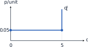
Each plantation can produce at most 5 pounds per day. Below $0.05 it produces nothing. At exactly $0.05 it is indifferent among all quantities from 0 to 5. Above $0.05 it produces at capacity:
One cane plantation\(q_c^s(p)=\begin{cases}0&p<0.05,\\ [0,5]&p=0.05,\\ 5&p>0.05.\end{cases}\)
Supply of one sugar cane plantation.
There are twenty plantations, so their combined supply is
All cane plantations\(Q_c^s(p)=\begin{cases}0&p<0.05,\\ [0,100]&p=0.05,\\ 100&p>0.05.\end{cases}\)
Sugar beet
A beet farm has variable cost \(q^2-0.9q\), a fixed cost of $1 and a subsidy of $1 per pound. We can treat the subsidy as a reduction in the farm's cost:
Cost after the subsidy\(C_b(q)\)\(=\)\(q^2-0.9q+1-q\)\(C_b(q)\)\(=\)\(q^2-1.9q+1\)
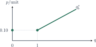
At the minimum of average cost, \(MC_b(q)=AC_b(q)\). This gives \(q^2=1\), so \(q=1\) and \(\min AC_b=AC_b(1)=0.10\). Above this threshold, setting \(p=MC_b(q)\) gives \(q=(p+1.9)/2\). The supply of one beet farm is
One beet farm\(q_b^s(p)=\begin{cases}0&p<0.10,\\ \{0,1\}&p=0.10,\\ \dfrac{p+1.9}{2}&p>0.10.\end{cases}\)
Supply of one sugar beet farm.
Adding the supplies of the 100 identical beet farms gives
All beet farms\(Q_b^s(p)=\begin{cases}0&p<0.10,\\ \{0,1,\cdots,100\}&p=0.10,\\ 50p+95&p>0.10.\end{cases}\)
Industry supply
Below $0.05, neither technology operates. At $0.05, the cane plantations can supply up to 100 pounds. Between $0.05 and $0.10, they supply 100 pounds while beet farms remain inactive. At $0.10, each beet farm chooses either zero or one pound. Above $0.10, beet output rises with price.